Zipf’s law in natural language

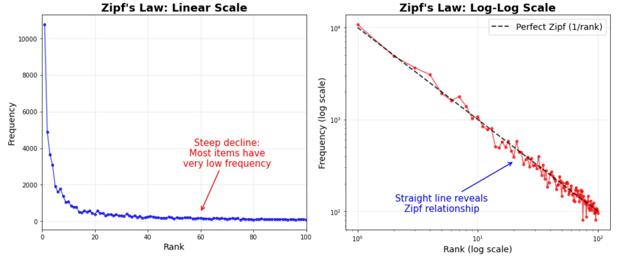
Nearly all modern optimizer benchmarks are run on natural language data, where token frequencies follow Zipf’s law^{22, 21}: the \(k\)-th most common token appears with frequency \(f(k)\propto 1/k^{\alpha}\) (\(\alpha\approx 1\)). A handful of tokens (“the”, “a”, “is”) dominate, while the vast majority of the ~100k vocabulary is rarely seen.

DNA is near-uniform

DNA, by contrast, has a vocabulary of just 4 nucleotides. In our training data (candidate cis-regulatory elements (cCREs) from ENCODE cell lines) the marginal nucleotide frequencies are strikingly close to uniform:

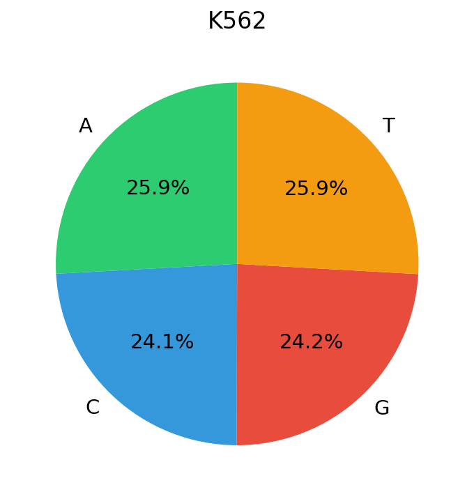
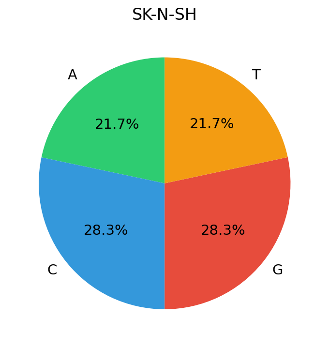
The entropy of DNA’s token distribution sits near its theoretical maximum: \(H_{\text{DNA}}\approx\log_2 4=2\) bits. Natural language, despite its vastly larger vocabulary, has lower normalized entropy because Zipf’s heavy tail concentrates probability mass on a small fraction of tokens. This distinction has concrete consequences for how optimizers see gradients, meaning the gradient statistics across tokens behave very differently numerically.

Optimizer performance is distribution-dependent

Wilson et al.²³ demonstrated empirically that the relative ranking of optimizers changes across domains: adaptive methods (Adam, AdaGrad, RMSProp) find solutions that generalize worse than SGD on image classification tasks, despite converging faster. Yet these same adaptive methods dominate SGD in language modeling, consistent with the classical No Free Lunch theorems²⁴, which prove that no single optimization algorithm is universally superior, and performance is always relative to the structure of the problem.

Our results extend this observation to genomics. The near-uniform token distribution of DNA removes the statistical asymmetry that adaptive methods exploit in NLP, while the low cardinality (\(K=4\)) and positional grammar of regulatory sequences create a loss landscape with fundamentally different curvature. This is precisely why benchmarking optimizers on DNA data directly (as we do here) is essential: rankings established on language corpora do not transfer.

While Adam¹ (see Appendix A) updates can lead to weight stagnation⁶⁷ and uneven signal propagation, Muon mitigates this by treating layers as matrices and “whitening”, or spreading out updates across singular dimensions to ensure all directions are learned with equal priority. Unlike Adam, which treats weights as flat vectors and risks remaining within the initialization neighborhood (closer to the NTK regime⁷), Muon forces weights to diverge from their starting points by distributing updates across the matrix space, thereby erasing initial distributions⁸. This is achieved by constraining all singular values of the weight updates to be close to \(1\), effectively “whitening” the update to distribute the learning signal evenly¹¹.

Just like Adam, we first form a momentum like exponential moving average of gradients, denoted by \(u_t\):

(with \(u_0=0\)). This plays the same role as Adam's first moment estimate \(m_t\), but is then processed using matrix structure. In our implementation we use Nesterov momentum¹Concretely, the input fed into the NS\(_5\) orthogonalization is not the raw gradient \(g_t\) but the lerp \((1-\beta)\,g_t + \beta\,u_{t}\). This Nesterov interpolation means the matrix that NS\(_5\) whitens is already a lookahead blend of the current gradient and the previous momentum buffer, not the gradient at \(W_t\) alone., so the input to the NS\(_5\) normalization is a lookahead lerp between the gradient and the momentum buffer, rather than the gradient at \(W_t\) alone.

We apply the SVD (see Appendix B) to the (momentum) update matrix \(u_t\): \[ u_t = U\Sigma V^\top. \] Muon constructs an update whose singular vectors match those of \(u_t\), but whose singular values are pushed toward \(1\): \[ \tilde u_t = U\,\tilde\Sigma\,V^\top, \] where \(\tilde\Sigma\) is a diagonal matrix with entries close to \(1\) (typically in \([0.7, 1.3]\)), projecting the update toward the Stiefel manifold²²The Stiefel manifold is the set of matrices with orthonormal columns (all singular values exactly equal to \(1\)). In practice, finite Newton-Schulz iterations only push singular values toward \(1\), not exactly to it. This is a stricter constraint than the Spectral Sphere, where only \(\sigma_1=1\) is constrained. “whitening” or “equalizing” the update across singular dimensions.

Intuitively, this prevents a few directions from dominating the step, and encourages motion in many independent directions of the layer's matrix space. In contrast to optimizers that treat parameters as a flat vector, Muon explicitly uses matrix structure, which can help avoid updates that remain concentrated near the initialization subspace.

In practice, the resulting parameter update has the form \[ W_{t+1} = W_t + U_t, \qquad U_t = -\eta\,\tilde u_t, \] (with optional weight decay applied as described in Appendix A).

Connecting Muon to norm control

Muon already manipulates singular values of the update (by pushing those of \(\tilde u_t\) toward \(1\)), which suggests a different view of regularization than standard weight decay. Classical weight decay controls the \(\ell_2\) or Frobenius norm of the weight matrices (defined as \(\|W\|_F =\|\vec W\|_2= \sqrt{\sum_{i}\sum_jw_{ij}^2}\)³\(\vec W\) denotes the vectorized form of matrix \(W\); more specifically, if \(W=[c_1, c_2, \dots, c_n]\) where \(c_i\) is the \(i\)th column of \(W\), then \(\vec W=\begin{bmatrix} c_1\\c_2\\\vdots\\c_n \end{bmatrix}\) has them merged into one column.⁴It also happens to be the case that \(\|W\|_F=\sqrt{\sum_i \sigma_i^2}\), but this is a bit of a digression and we will not prove this here.), but in a matrix aware setting one can instead target properties tied to singular values:

• Rank / intrinsic dimension: shaping the smaller singular values can encourage using many subspaces of the hidden stream, rather than collapsing the layer to an effectively low rank map.
• Stability: bounding the largest singular value (the spectral norm) controls the layer Lipschitz constant, and helps prevent activation and gradient blowups^{12, 115}Concretely, if all singular values of the update equal \(1\), then \(\tilde u_t\) is orthogonal and \(\|\tilde u_t\, x\| = \|x\|\) for every input \(x\) (provided \(\tilde u_t\) is square). More generally, \(\|\tilde u_t\, x\| \leq \sigma_1(\tilde u_t)\,\|x\|\), so pushing \(\sigma_1\) toward \(1\) directly caps the maximum activation amplification per layer..

This perspective is especially relevant for high dimensional, structured sequence representations like DNA. The combinatorial grammar of regulatory motifs demands that many spectral dimensions remain active; a low rank collapse in the update would erase the subtle, distributed signals that distinguish functional sequences from background.

To isolate the effect of the optimizer, we hold model architecture, dataset, training duration, and all non-optimizer hyperparameters constant across runs, varying only the optimizer and learning rate. We track validation perplexity throughout training as a highly interpretable and sensitive measure of model capacity⁸The model is a multifunctional architecture similar to Axis, trained on a set of candidate cis-regulatory elements (cCREs) from the ENCODE v4 registry that are cell-type-specific to one of three cell lines: K562, HepG2, and SK-N-SH. Training was limited to 20 epochs due to compute constraints; the loss has not begun to saturate (we have trained to much lower cross-entropy in prior runs), so these results reflect relative optimizer comparisons, not absolute model quality.. We use perplexity as a sensitive proxy for sequence modeling quality; in practice we expect improvements to correlate with better motif and grammar modeling, and we plan to validate this directly with motif-centric downstream tasks. By evaluating against a held-out validation split, we extract a clear empirical picture of optimizer performance across varying learning rates and training checkpoints (saved every epoch).

Final test perplexity by learning rate

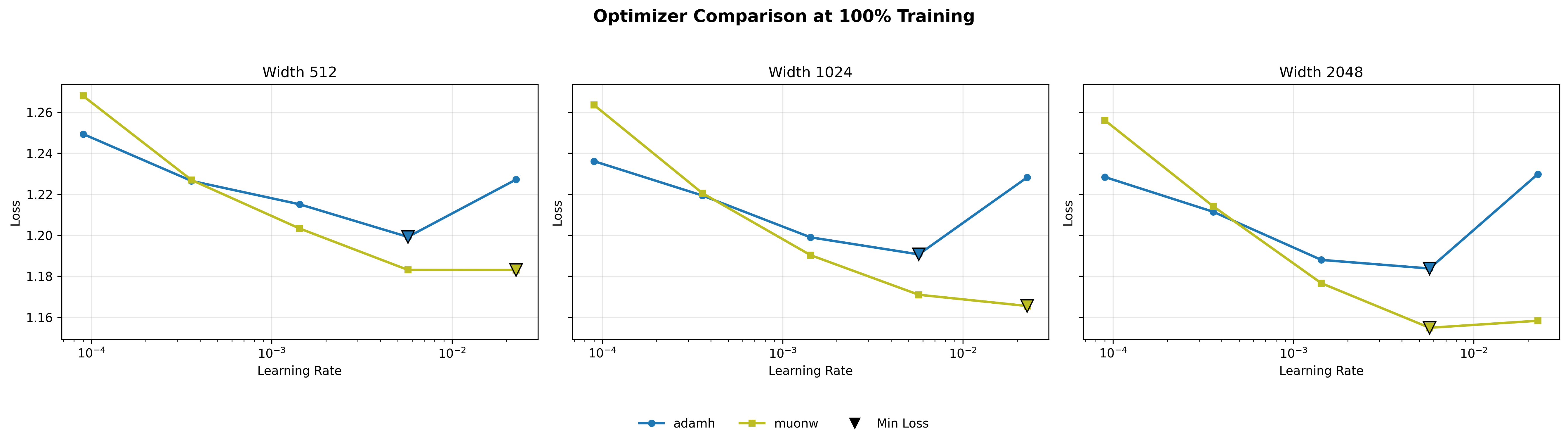
The line plots below illustrate the final validation perplexity (at the last checkpoint) for each optimizer pair as a function of the learning rate (log scale). Lower perplexity indicates superior probability mass placement on the target sequence.

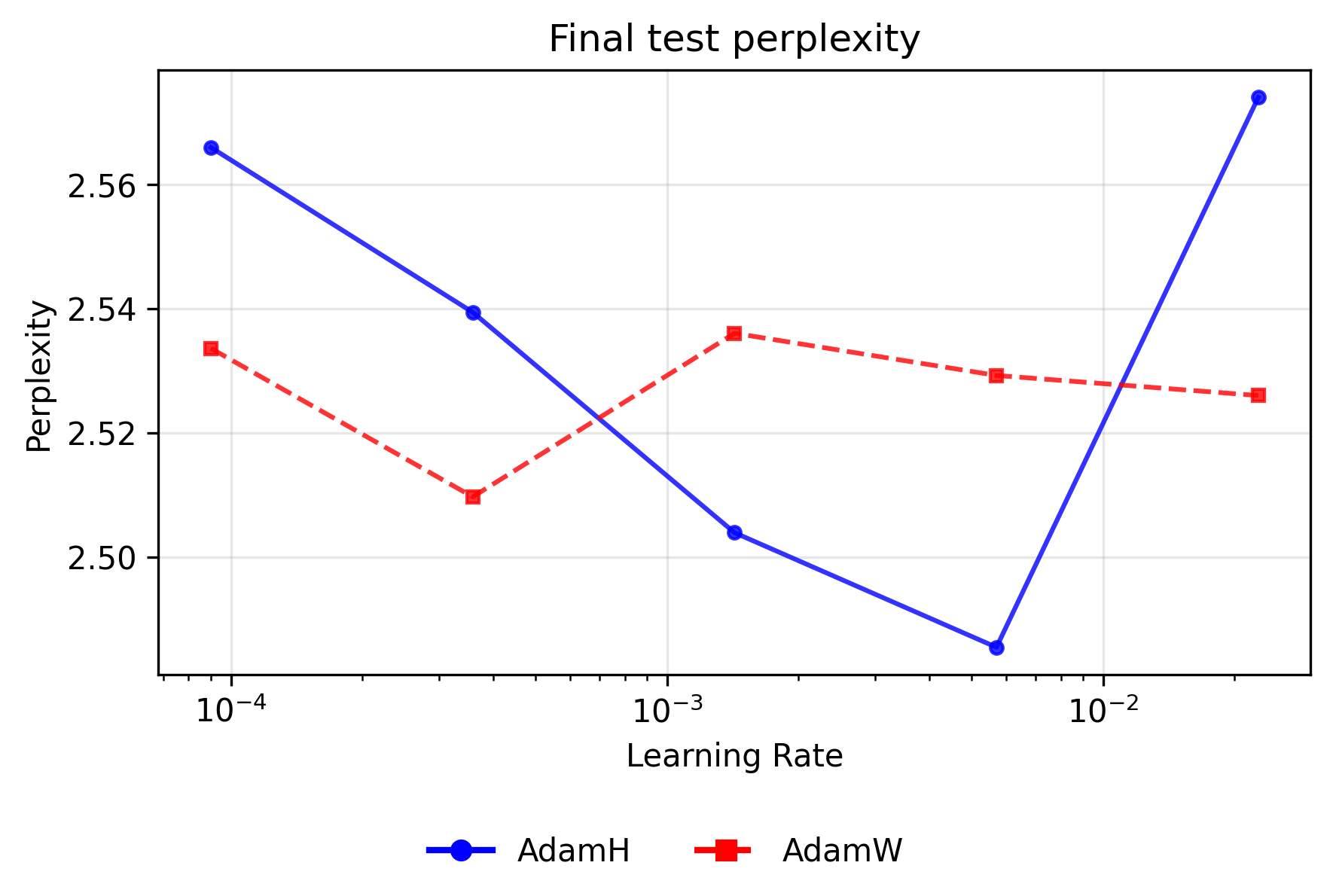
For Adam variants, applying the Hyperball constraint improves peak performance but sharply narrows the stable operating window. AdamH achieves the absolute lowest overall perplexity for the Adam family (∼2.485) at a moderate learning rate of ∼\(5.69 \times 10^{-3}\). However, AdamW proves dramatically more resilient at the extremes. At the lowest learning rate (∼\(9.00 \times 10^{-5}\)), AdamW's independent weight decay slowly regularizes the network without disrupting the coordinate-wise updates, maintaining a lead (∼2.534 vs. ∼2.566). Conversely, at the highest rate (∼\(2.27 \times 10^{-2}\)), AdamH degrades sharply (∼2.574); its rigidly fixed norm overrides the natural decay in step size that occurs when weights grow, causing the optimizer to catastrophically bounce around the local minimum, while AdamW remains relatively stable (∼2.526).

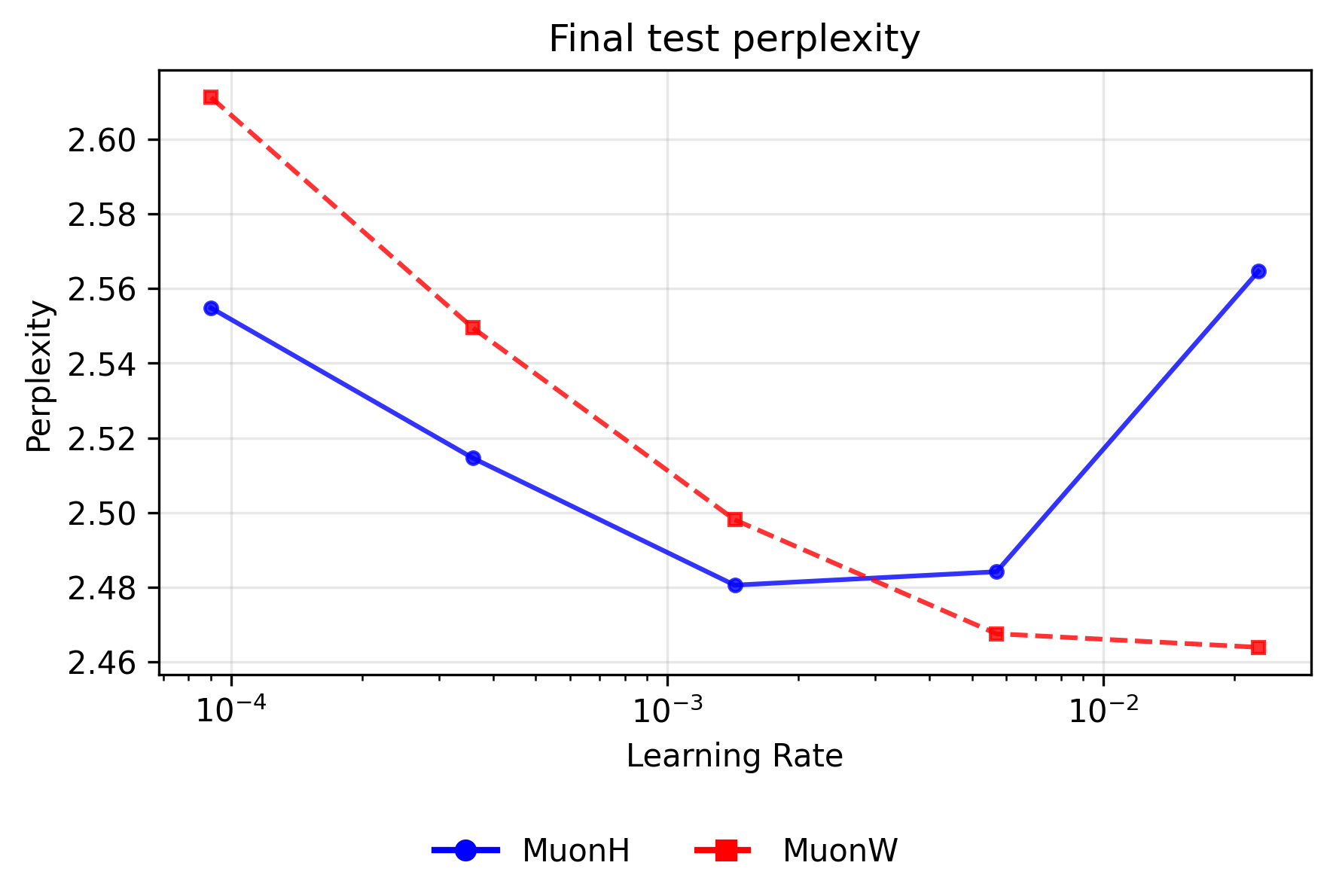
The dynamics for the Muon optimizers are perfectly inverted: Hyperball dominates at lower learning rates, whereas independent weight decay scales flawlessly to the highest rates. Because Muon's whitened updates are entirely scale-free, MuonW relies on the unbounded growth of the weight norm to act as an implicit learning rate scheduler (decreasing the relative step size over time). At higher learning rates (∼\(2.27 \times 10^{-2}\)), this rapid norm growth naturally cools the optimization, allowing MuonW to comfortably digest large initial steps and achieve the absolute best validation perplexity across all sweeps (∼2.464). MuonH’s fixed norm eliminates this vital annealing phase, permanently trapping it in a high-temperature regime and causing perplexity to rise (∼2.565). Conversely, at small learning rates like ∼\(9.00 \times 10^{-5}\), where preventing further step-size decay is actually beneficial, MuonH easily outperforms MuonW.

Overall findings

These validation results, together with the training loss curves below, paint a consistent picture: the Hyperball constraint does not uniformly improve both optimizers, and the best overall configuration is Muon with independent weight decay (MuonW)⁹The Hyperball blog¹⁰ actually shows that for Muon, the losses are comparable for models with ≤ 500M parameters, and Hyperball dominates for the largest model of >1B parameters. Our largest model is actually ~420M parameters large (as we are somewhat compute bound), so it is still possible for MuonH to outperform MuonW at a larger scale..

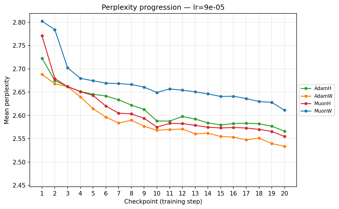
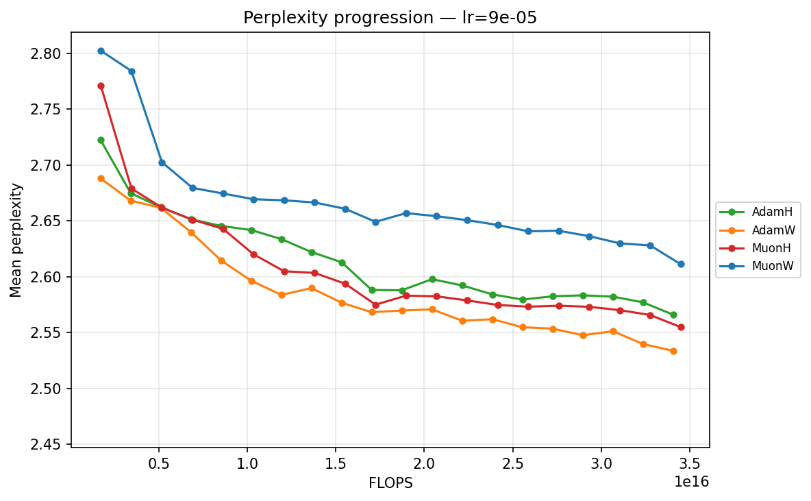
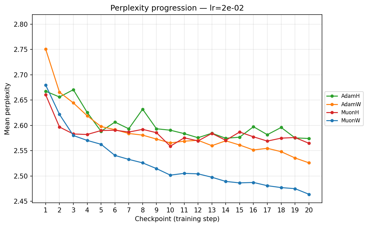
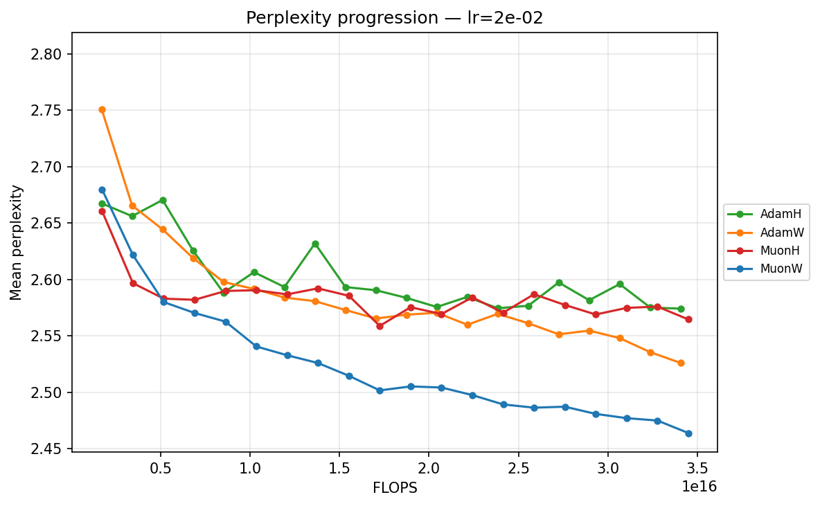
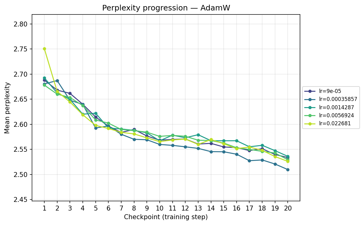
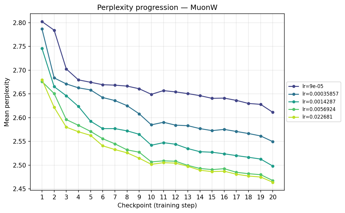
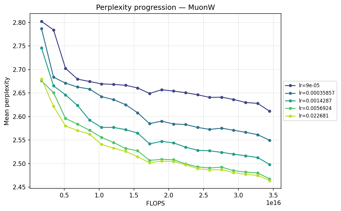
Perplexity progression by checkpoint and FLOPS

To understand the temporal dynamics behind the final results, we track the mean validation perplexity over the 20 checkpoints. Because validation perplexity can be volatile, observing its trajectory provides crucial context about optimizer stability and the risk of overfitting. We present each progression in two views: by training step (checkpoint) and by total FLOPS. The FLOPS axis accounts for the per-step compute cost of each optimizer, including forward/backward passes and the optimizer update itself (e.g. Muon's SVD is more expensive per step than Adam's elementwise update). We can view this progression from two perspectives: comparing optimizers at each learning rate, and comparing learning rates for each optimizer.

First, we slice the data by learning rate, placing all four optimizers head-to-head at each scale:

By checkpoint

By FLOPS

lr ≈ 9.00×10⁻⁵

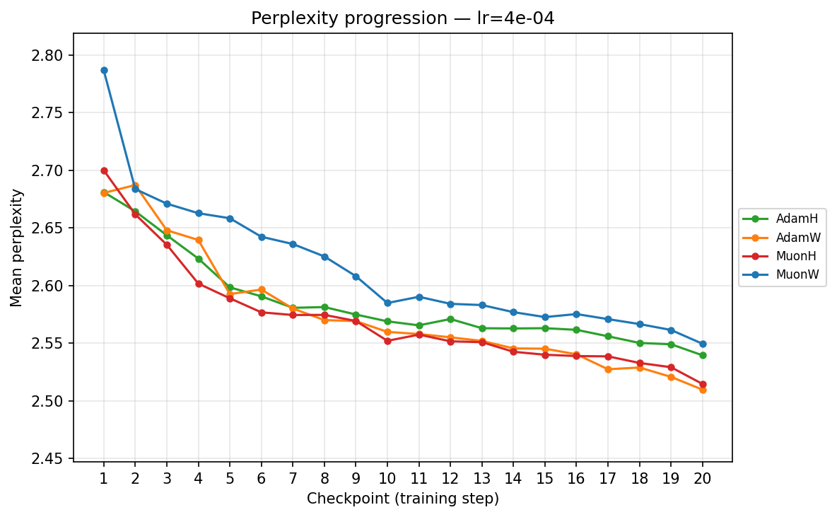
lr ≈ 3.59×10⁻⁴

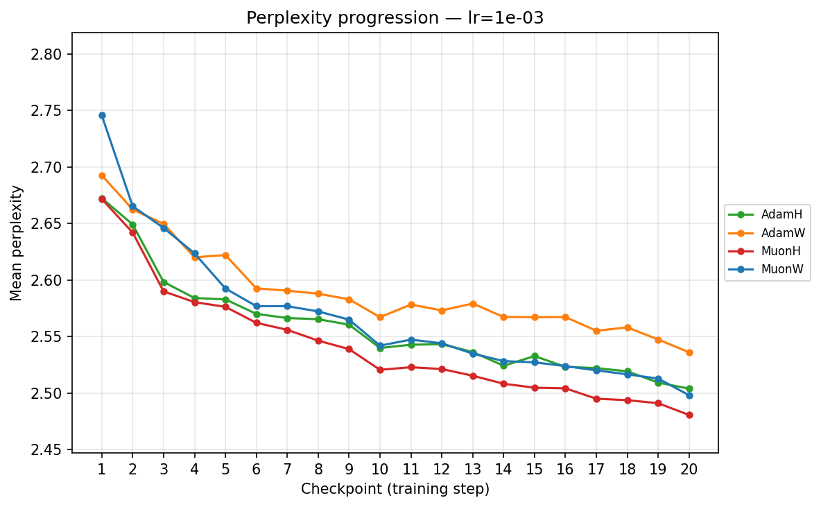
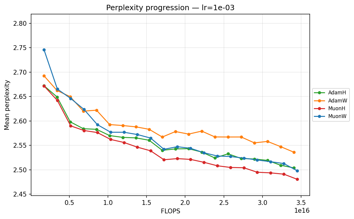
lr ≈ 1.43×10⁻³

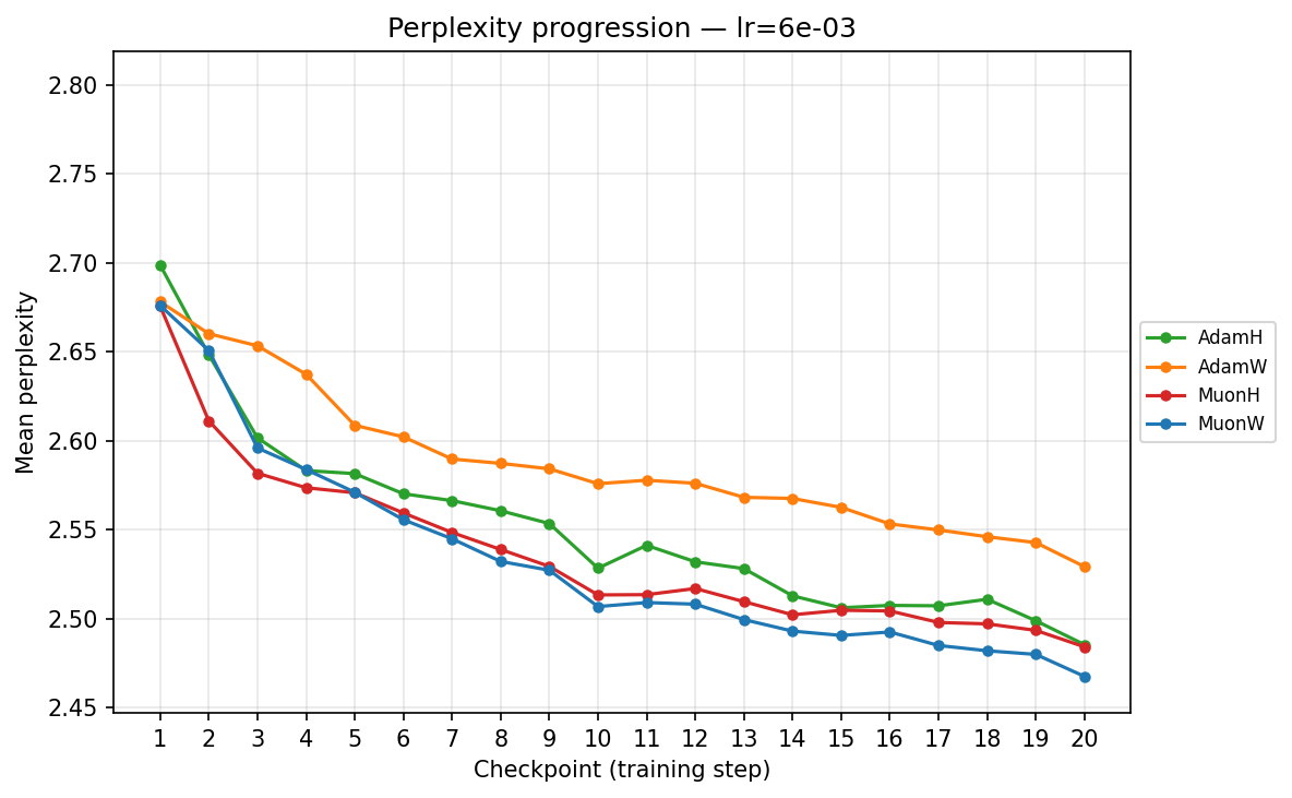
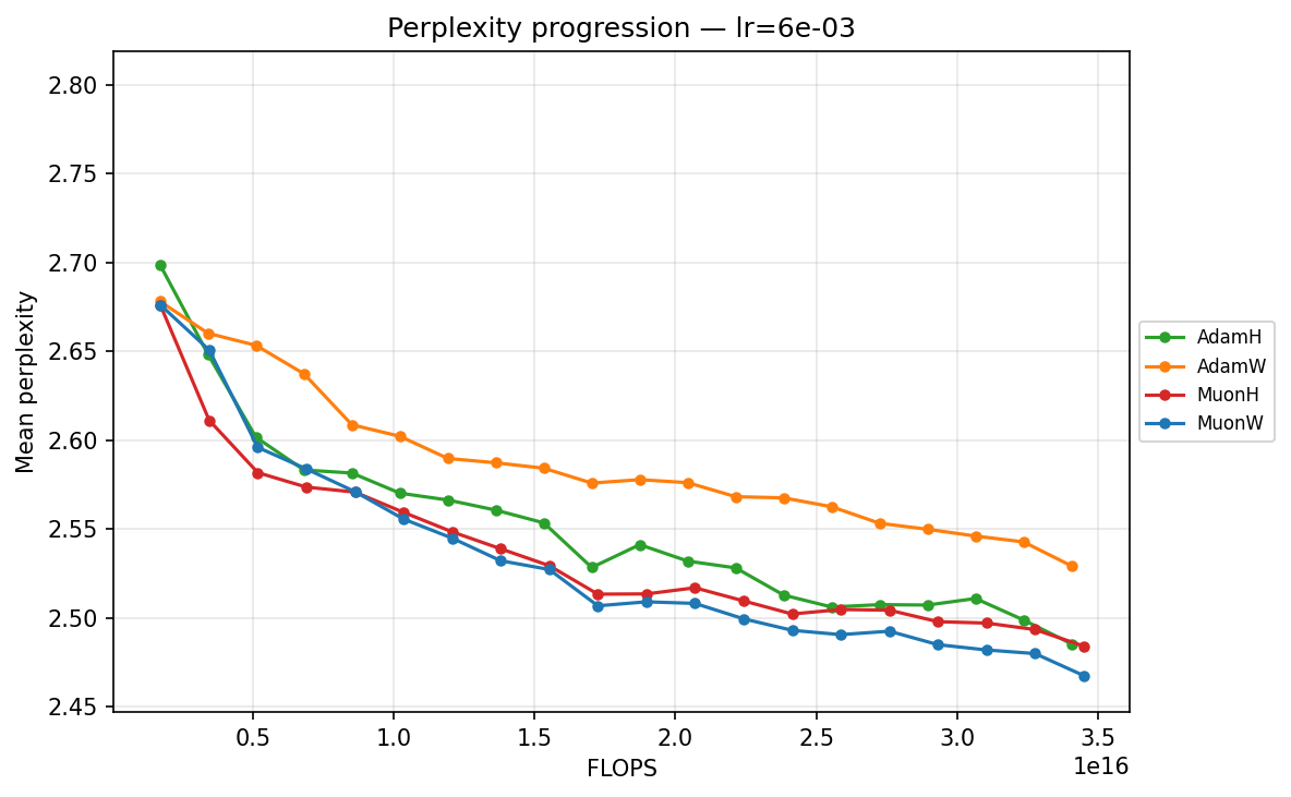
lr ≈ 5.69×10⁻³

lr ≈ 2.27×10⁻²

Analyzing these cross-sections reveals a clear shifting of the guard as the step size scales up:

• Low Learning Rates (∼\(9.00 \times 10^{-5}\) to ∼\(3.59 \times 10^{-4}\)): Training is slow but highly stable. Here, the strict norm constraints of Hyperball provide a massive early acceleration. MuonH drops aggressively in the first few epochs, cleanly outperforming MuonW, which converges much more deliberately. AdamH, strangely, struggles at the absolute lowest rate compared to AdamW, but tightens the gap as the LR increases.
• Mid-Range (∼\(1.43 \times 10^{-3}\) to ∼\(5.69 \times 10^{-3}\)): We enter the optimal operating window for most models. At ∼\(5.69 \times 10^{-3}\), AdamH finally hits its stride, overtaking AdamW to reach the lowest perplexity in the Adam family. Concurrently, MuonW overtakes MuonH. MuonW leverages the larger step size perfectly, free from the norm bound that begins to bottleneck MuonH's performance.
• High Learning Rate (∼\(2.27 \times 10^{-2}\)): We observe sharp destabilization for fixed-norm constraints (AdamH, MuonH); their trajectories bounce erratically and plateau at suboptimal levels, likely due to how hard constraints interact with high-variance updates. In stark contrast, MuonW thrives, plunging rapidly to achieve the absolute lowest validation perplexity (∼2.464) across all runs. AdamW remains remarkably resilient but reaches higher validation perplexity than MuonW, suggesting that MuonW achieves higher effective capacity in this regime.

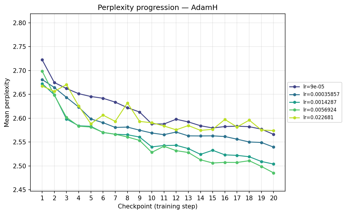
Next, we transpose the axes to view the same data grouped by optimizer, illustrating their individual hyperparameter sensitivities:

By checkpoint

By FLOPS

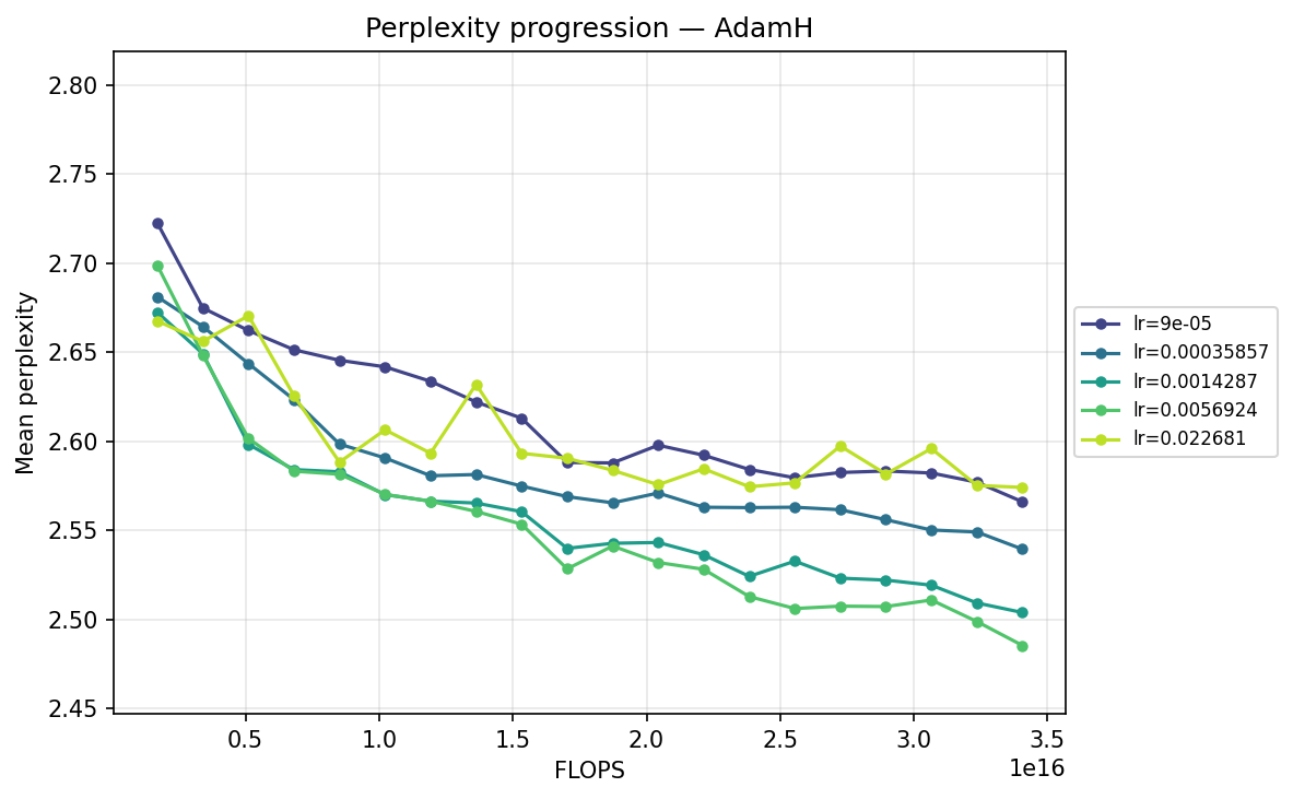
AdamH

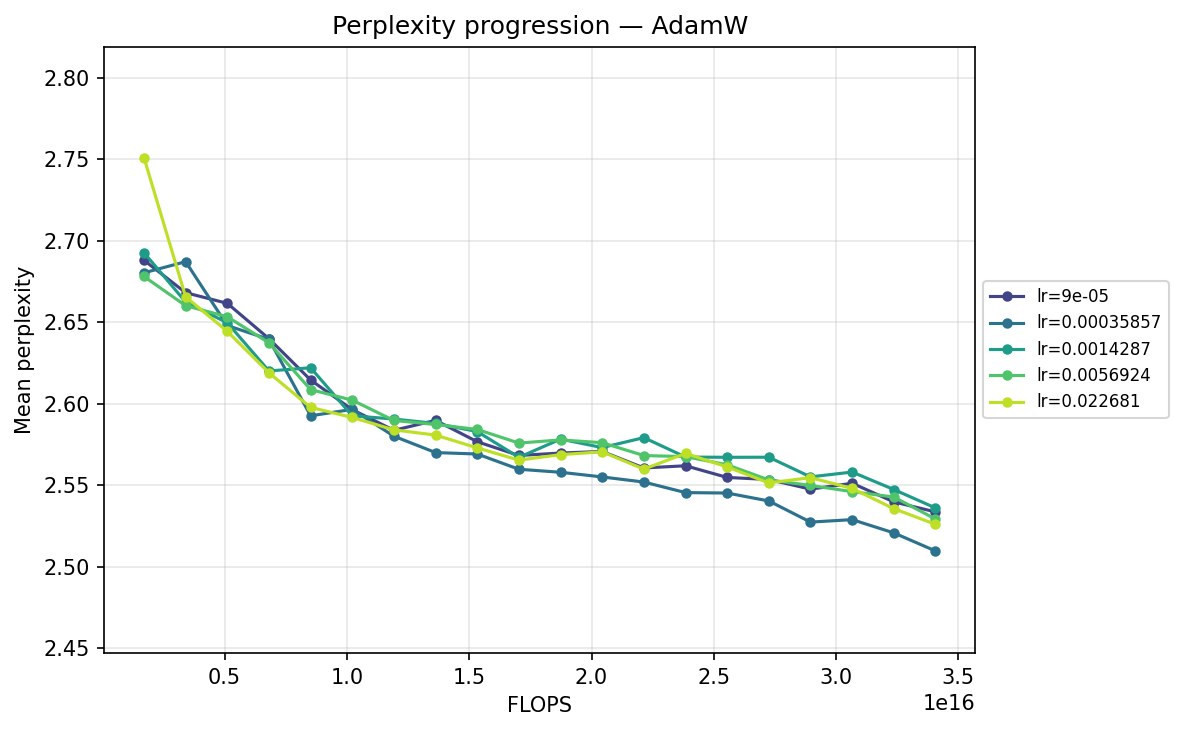
AdamW

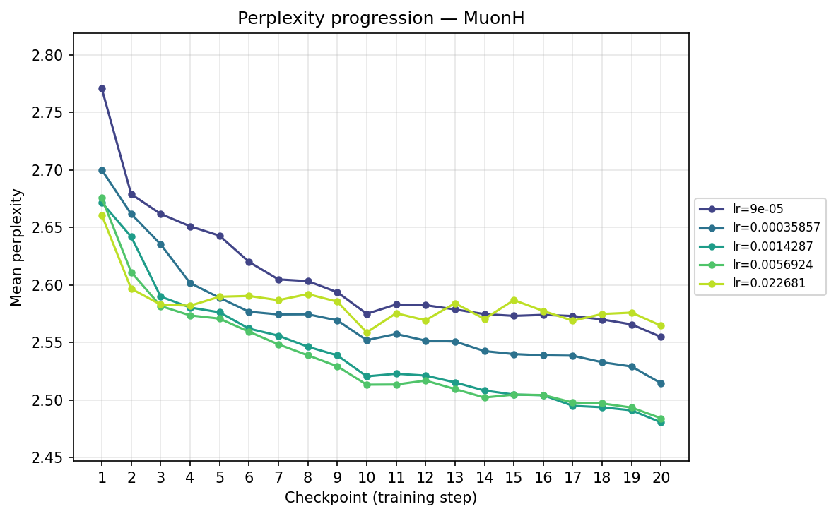
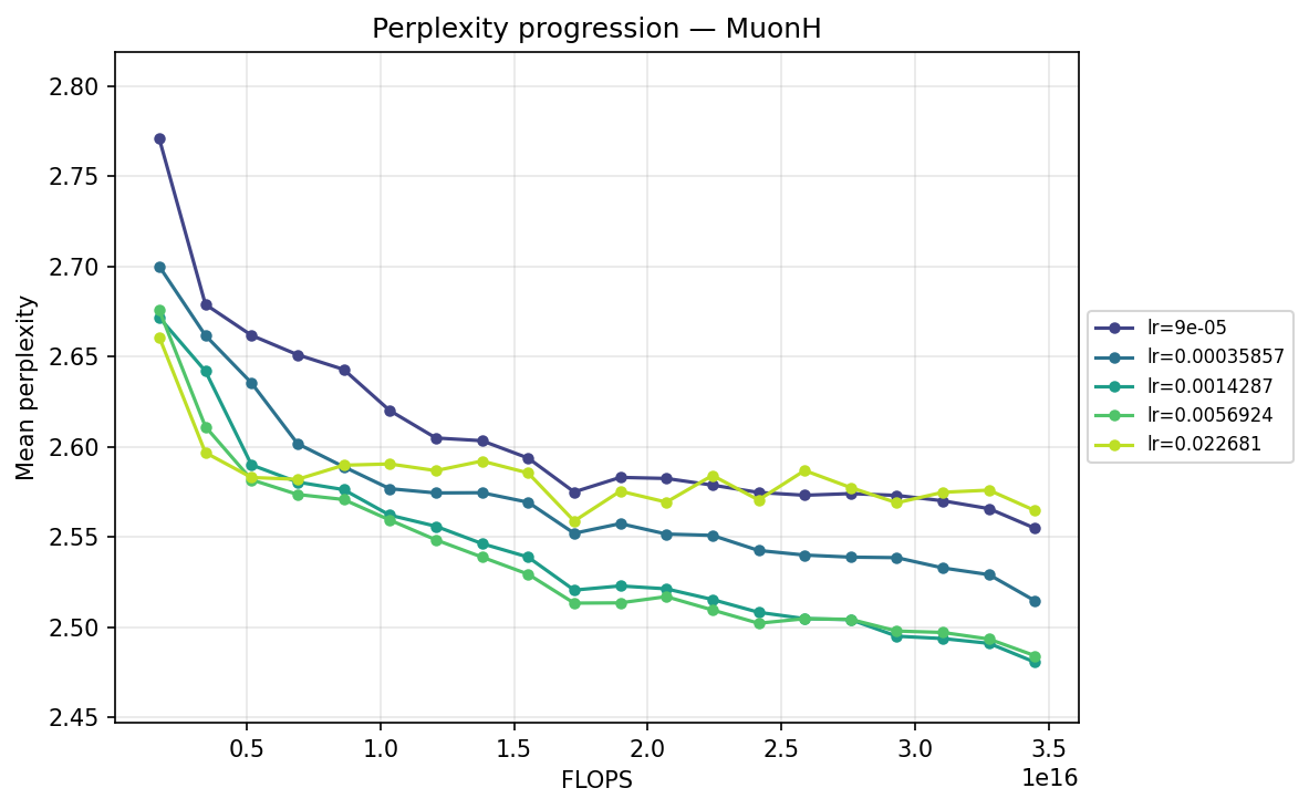
MuonH

MuonW

Viewing the optimizers individually clarifies these dynamics. For AdamH, the intermediate learning rate ∼\(5.69 \times 10^{-3}\) (yellow) provides the steepest drop and lowest final perplexity (∼2.48). Exceed this, and it destabilizes; fall short, and it converges too slowly. AdamW is far more forgiving across learning rates: at \(\approx 3.59 \times 10^{-4}\), it settles into a remarkably smooth, steady decline to its lowest perplexity of ∼2.51. MuonH exhibits a narrow but highly effective sweet spot at mid-range LRs (∼\(1.43 \times 10^{-3}\) to ∼\(5.69 \times 10^{-3}\)), but is heavily penalized at the maximum rate. Finally, MuonW distinctly favors scale: its progression monotonically improves as the learning rate increases, with the highest LR (∼\(2.27 \times 10^{-2}\)) driving the lowest perplexity overall.

Time-to-target: FLOP efficiency

We can quantify optimization efficiency by measuring the training FLOPs required to cross a specific validation target. We use a target of 2.51, the lowest perplexity reached by an optimizer candidate (specifically AdamW). MuonW at its optimal learning rate crosses this threshold by checkpoint 12, while AdamH at its optimal configuration only reaches it around checkpoint 19. This means MuonW reaches the target in roughly 37% fewer steps (and 37% fewer training tokens). Because the forward and backward passes dominate per-step FLOPs, Muon’s SVD-based update adds only a small overhead relative to the total step cost, so the 37% step reduction translates to a comparable reduction in total training FLOPs.

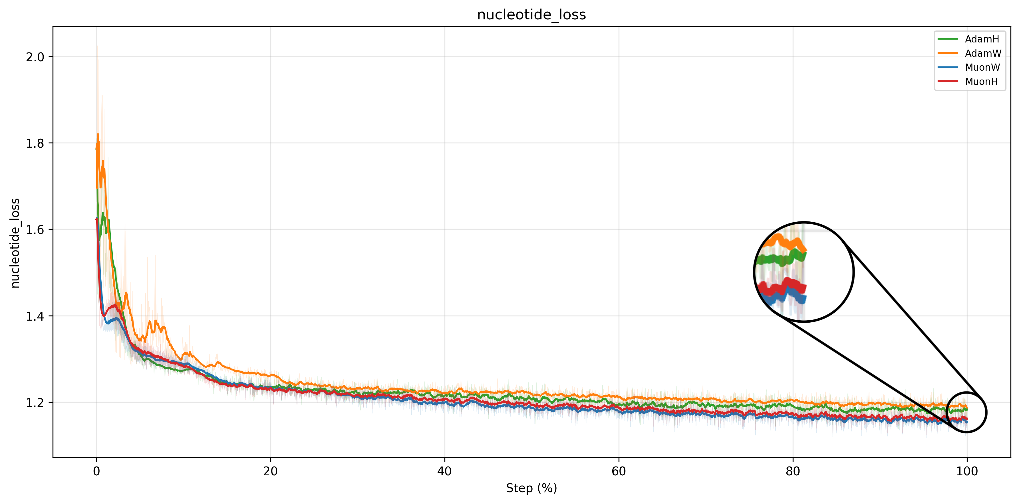
Consistent with existing literature²¹⁰, Muon achieves a lower train loss than Adam across all configurations. The loss curves confirm the ranking established by the validation perplexity above: MuonW converges fastest and reaches the lowest loss, followed by MuonH, AdamH, and AdamW.

Learning rate sweep analysis

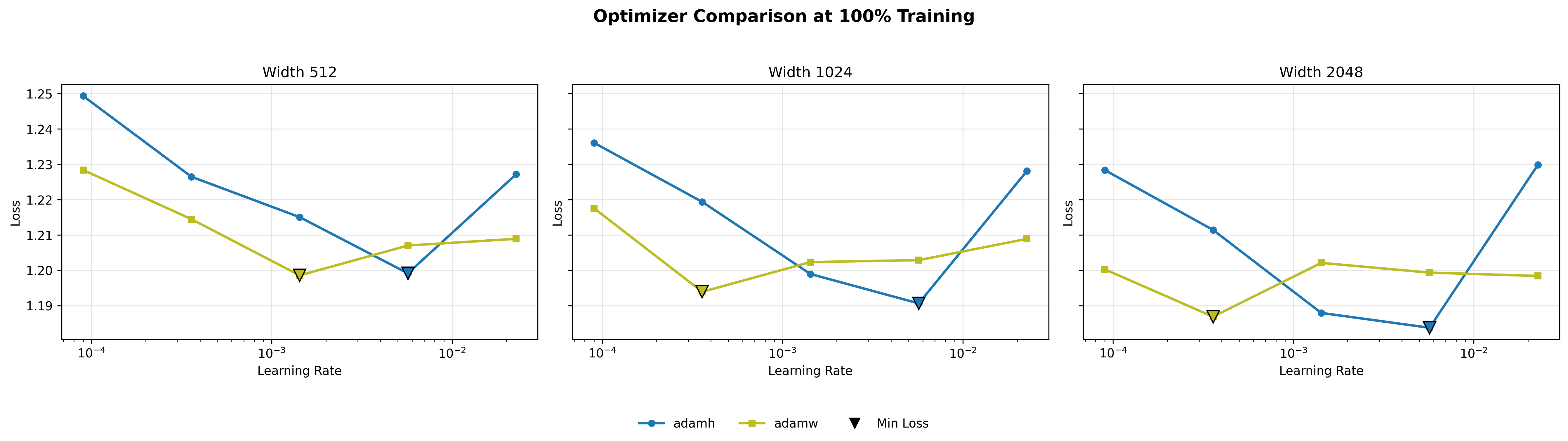
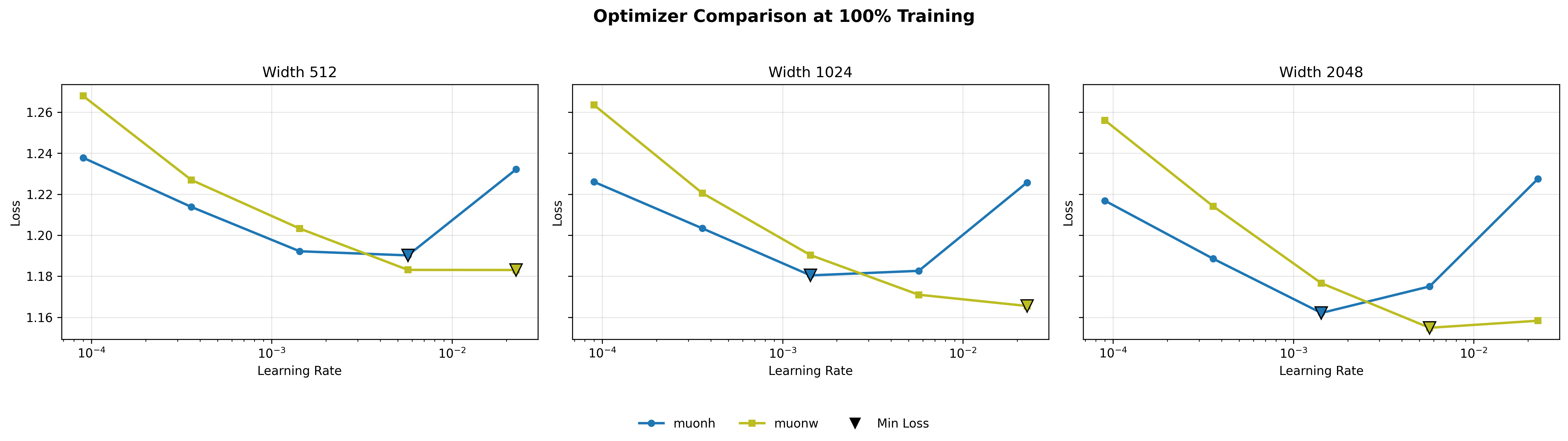
What is striking about these sweep curves is how consistent their structure is across scales. For Adam, Hyperball (blue) carves out a partial convex basin in the mid learning rate range (\(\sim 10^{-3}\) to \(10^{-2}\)), dipping below weight decay (yellow) in that region and rising above it at both extremes. This shape persists across widths, suggesting that Hyperball’s norm control is genuinely helpful in Adam’s optimal operating range. For Muon, the pattern is different: MuonW’s (yellow) loss decreases roughly linearly with increasing step size, while MuonH (blue) curves downward then upward more sharply. MuonW reaches a lower minimum at a higher learning rate. This near-linear response for MuonH also holds across scales, hinting that Hyperball’s fixed-norm constraint limits how much Muon can exploit larger step sizes.

For Adam, the lowest point is with Hyperball at \(\eta \approx 5.69 \times 10^{-3}\) (compared to AdamW at \(\approx 3.59 \times 10^{-4}\)). For Muon, the lowest point is generally achieved with weight decay at the higher end of tested learning rates, scaling up to \(\eta \approx 2.27 \times 10^{-2}\) (although Hyperball reaches its optimum earlier at \(\eta \approx 1.43 \times 10^{-3}\)). This disparity highlights a key distinction: while Adam's coordinate-wise updates become highly unstable at large learning rates, Muon's whitened updates, when unconstrained by a fixed norm, can safely exploit much larger step sizes to drive down the loss.

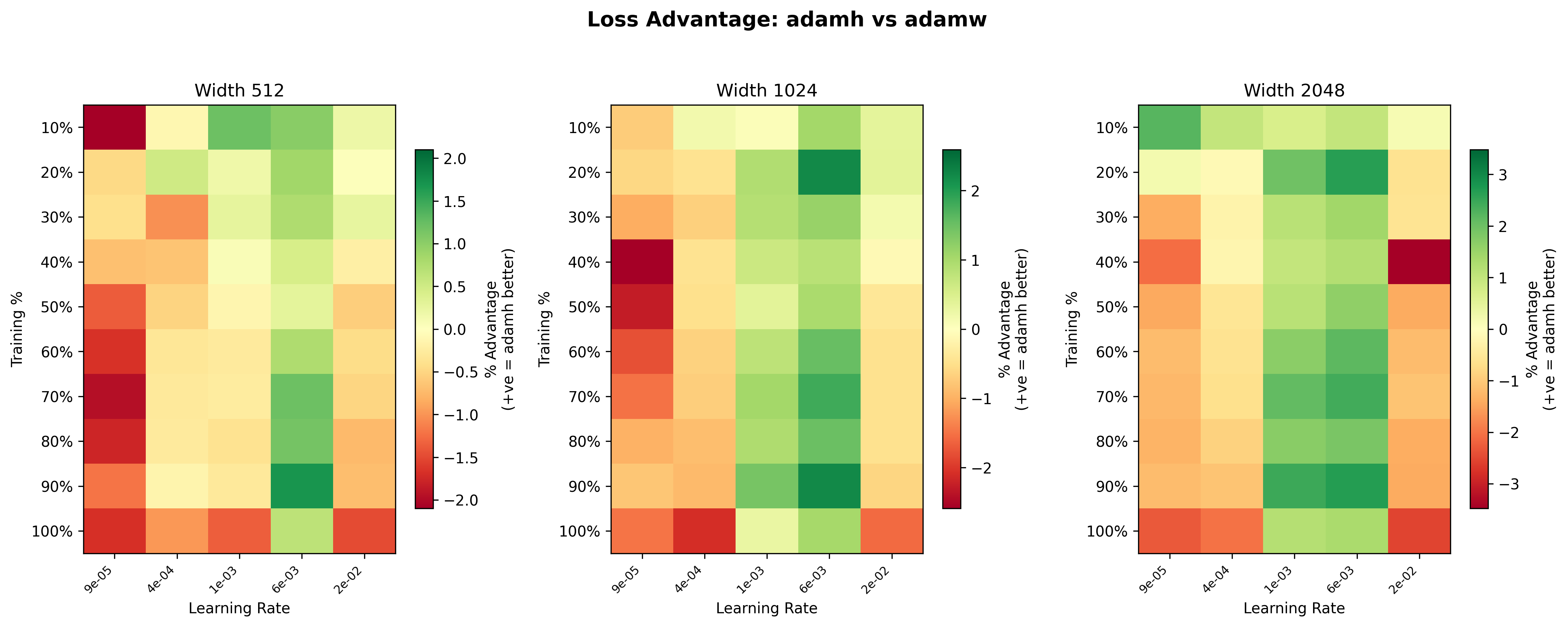
These heatmaps¹¹Each heatmap uses its own color scale, so the same shade of green or red can represent different magnitudes across panels. Pay attention to the individual legends. give us a clearer picture of where Hyperball (blue) has the advantage over weight decay (yellow). For Adam, the advantage is scale-dependent: at width 512, the heatmap is mostly yellow (roughly even), but at width 2048, AdamH shows a noticeably stronger advantage, with greener squares across much of the grid. In particular, the mid learning rate range (\(\sim 10^{-3}\) to \(6\times 10^{-3}\)) is consistently green across widths, suggesting Hyperball’s norm control is most beneficial at moderate step sizes. At the highest learning rate (\(2.27\times 10^{-2}\)), weight decay dominates, likely because the effective step size grows too large (it grows \(\propto\eta\)) and training can never stabilize.

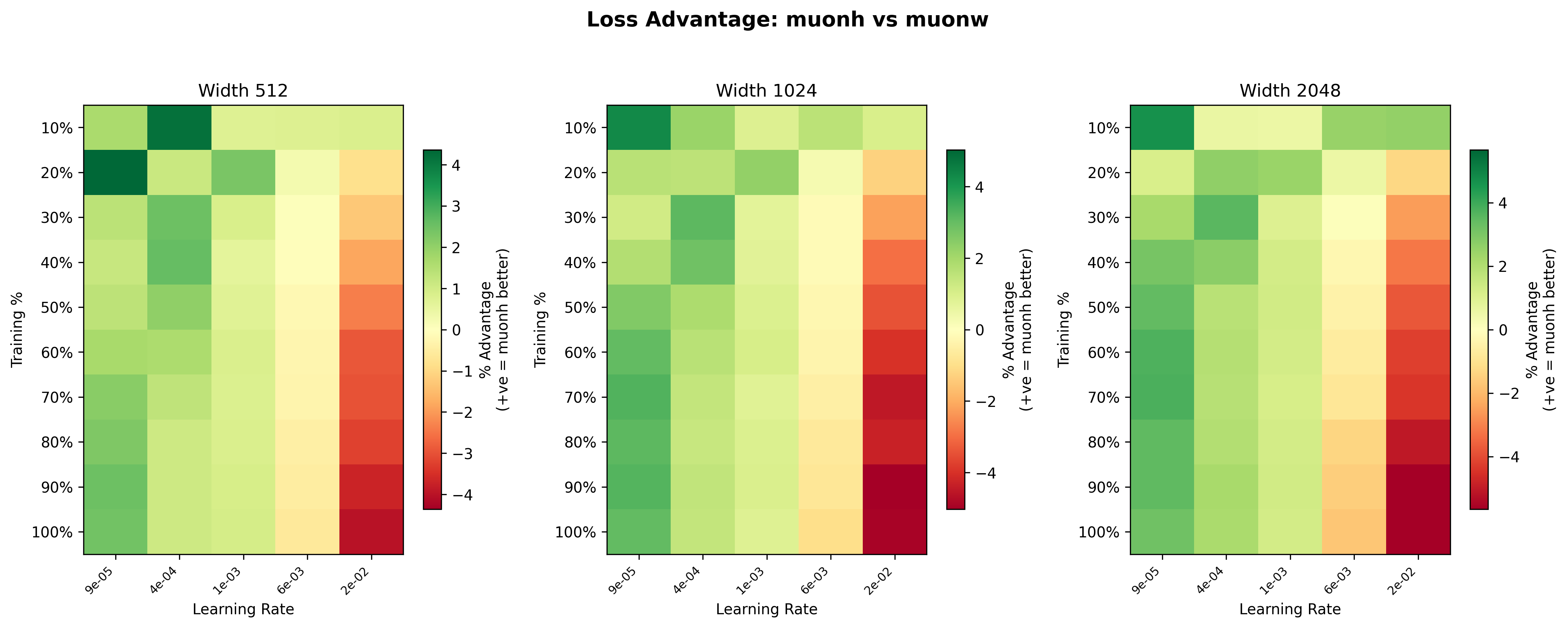
For Muon, the scale dependence runs in the opposite direction. At width 512, Hyperball is competitive or slightly ahead across much of the grid, with light green dominating the mid learning rates. By width 1024, the advantage fades to mostly yellow, and at width 2048 the picture inverts: the heatmap is mostly warm, with weight decay winning by up to ~4.5% at the higher learning rates late in training. This suggests that the spectral squeeze (described in the Spectral Analysis) worsens with scale; larger weight matrices have more trailing singular directions for the uniform rescaling to erode.

Cross-optimizer comparison

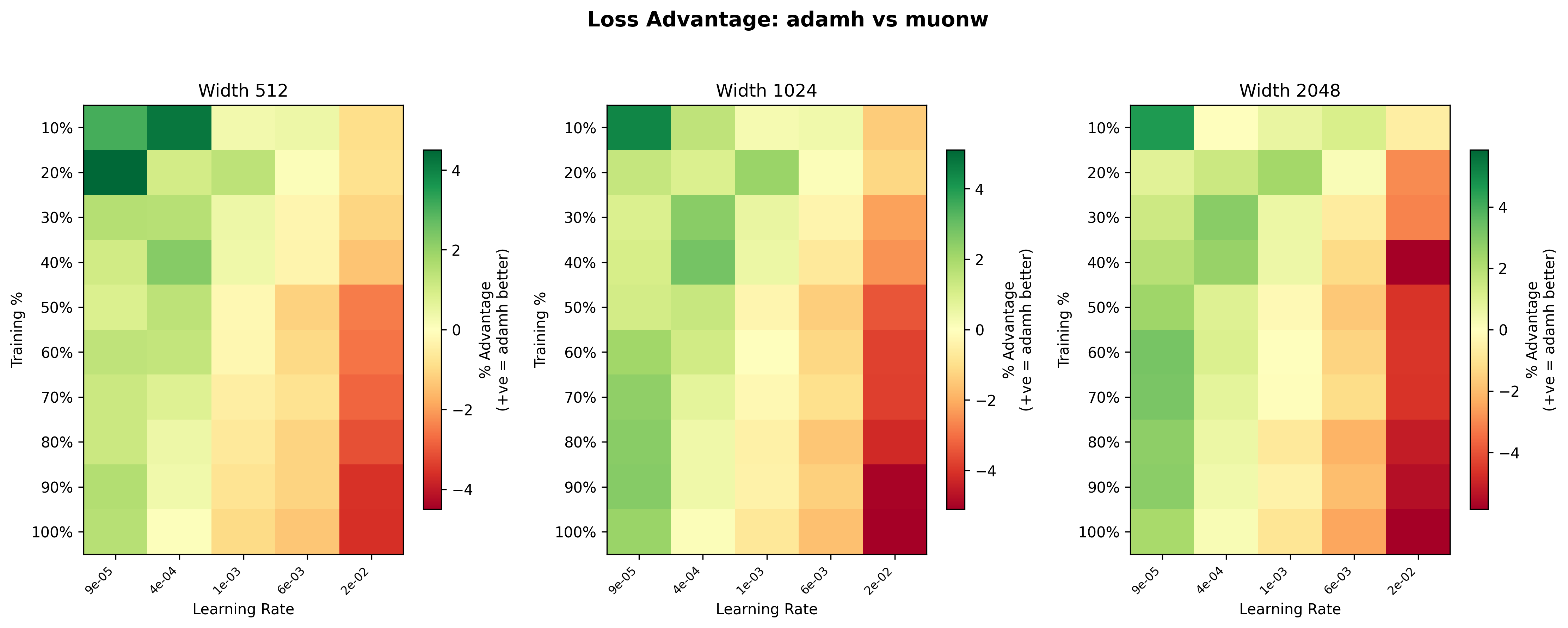
Finally, we compare the two best configurations head-to-head: MuonW against AdamH. Even at width 512, MuonW eventually pulls away; the curves track each other at lower learning rates, but MuonW pulls away at higher learning rates. What changes with scale is consistency: at width 1024 and especially 2048, AdamH holds the advantage across the broader low/mid range, while MuonW dominates the high learning rate extremes by a massive margin. The loss curves reinforce this: the gap between blue and yellow widens at higher learning rates and persists more uniformly at larger widths, suggesting that the performance gap increases with width, consistent with a spectral mechanism discussed below.

To understand why Muon with independent weight decay (MuonW) outperforms its constrained counterpart (MuonH), we can gain insight by examining the spectral properties of the learned representations. Rather than examining the spectral norm itself (since the exact multiplier is less important given scale invariance), we focus on the distribution of singular values. Following the eigenspectral framework of NerVE¹⁵¹²NerVE originally applies these metrics to track activation dynamics through FFN layers, but the same spectral measures are equally well defined for weight matrices., we track two key metrics for the weight matrices:

• Spectral Entropy: A measure of how uniformly variance is distributed across singular values. Values near \(1.0\) indicate a "full rank", diverse representation, while values near \(0\) indicate rank collapse (variance concentrated in a few dimensions).
• Participation Ratio (PR): The effective rank of the matrix. Higher PR means more active dimensions are used to represent data. We normalize the PR to get the ratio of the effective rank to full rank, which allows us to compare matrices of different shapes (we want to see the training dynamics, exact scale is not important).

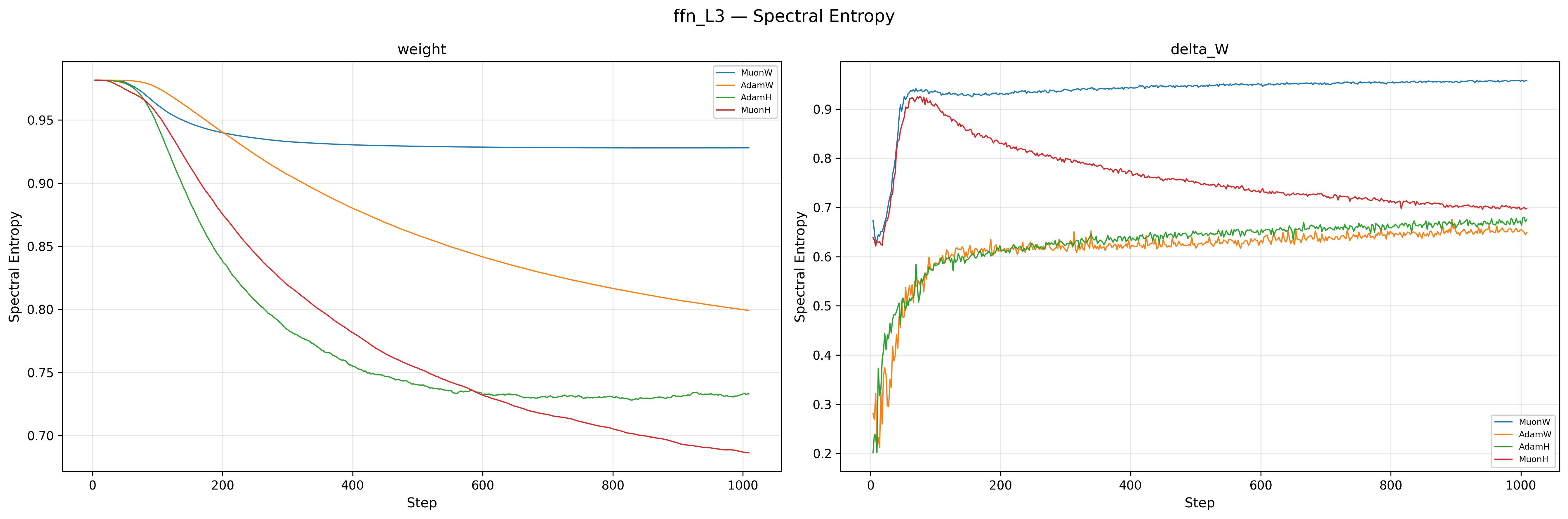
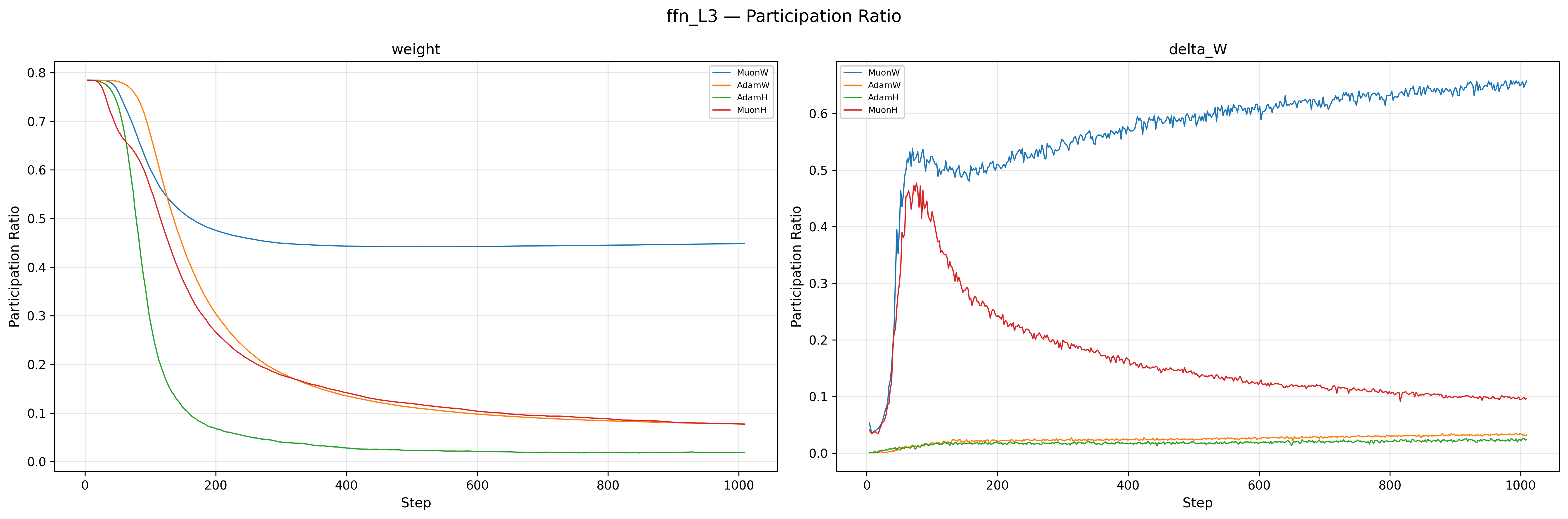
The weights of MuonW (Blue) and MuonH (Red) both start with high spectral entropy (\(\approx 0.98\)), but their trajectories diverge sharply. MuonW’s entropy decreases only slightly and stabilizes near \(\approx 0.93\), indicating that the weight matrices maintain a near-uniform singular value distribution throughout training; this is consistent with whitened updates supporting a more distributed spectral structure. MuonH (Red), by contrast, steadily collapses from \(\approx 0.98\) to \(\approx 0.68\), with the participation ratio falling in tandem: the effective rank of the weight matrices shrinks over training, a strong rank/entropy collapse signature that could indicate representational degeneration¹⁶. The Adam variants (Orange, Green) sit relatively lower for delta_W, which is expected since Adam does not whiten its updates. The critical observation is the divergence between Blue and Red: both use the same Muon whitening, yet MuonH’s spectrum degrades while MuonW’s does not. This is strongly consistent with the Hyperball constraint driving the degradation. The \(\Delta W\) entropy tells a consistent story: MuonW’s updates rise and stabilize near \(\approx 0.95\), while MuonH’s updates peak early and then become progressively less whitened (dropping from \(\approx 0.92\) to \(\approx 0.7\)), consistent with a feedback loop from the weights into the updates.

Uniform Rescaling and the Spectral Squeeze

MuonH (Red) constrains \(\|W\|_F = R\) at every step by multiplying every singular value by the same factor \(c = R/\|W_t + U_t\|_F\). The large singular values survive this downscaling; the small ones (which Muon’s whitening tried to grow) cannot, because the uniform rescaling pulls them back down before they accumulate meaningful energy. Over many steps this concentrates the spectrum into fewer dominant modes, erasing the weak regulatory signals in the tail.

This effect is compounded on the update side. Recall that Muon’s NS\(_5\) whitening is imperfect: it pushes singular values toward \(1\) but lands in roughly \([0.7, 1.3]\), not exactly at \(1\). For MuonW (Blue), these small imperfections are benign; the weight matrix is free to absorb them, and the \(\Delta W\) spectral entropy stays high (\(\approx 0.95\)) throughout training. For MuonH (Red), one plausible mechanism is a feedback loop: as the weight spectrum collapses, the gradients computed at \(W_t\) become increasingly anisotropic, which flows into the momentum buffer. Imperfect NS\(_5\) whitening may be insufficient to fully recover a uniform spectrum from this biased input, so the update itself becomes progressively less whitened. In the \(\Delta W\) entropy plot, MuonH (Red) starts near MuonW (Blue) but steadily diverges, dropping to \(\approx 0.7\) by the end of training, consistent with this hypothesized mechanism.

In contrast, MuonW (Blue) imposes no hard constraint on the weight norm, so there is no uniform rescaling step and no feedback loop. Muon’s whitened updates can grow the small singular directions over many steps without them being pulled back, and the dominant singular directions can grow without suppressing the smaller ones. MuonW shows sustained higher spectral entropy and participation ratio, suggesting a more distributed use of singular directions; we hypothesize this helps increase capacity and retain combinatorial regulatory structure.

Implicit Annealing and Relative Step Size

The second piece of the puzzle lies in the relative step size. We define the relative step size as \(\frac{\|\Delta W\|}{\|W\|}\).

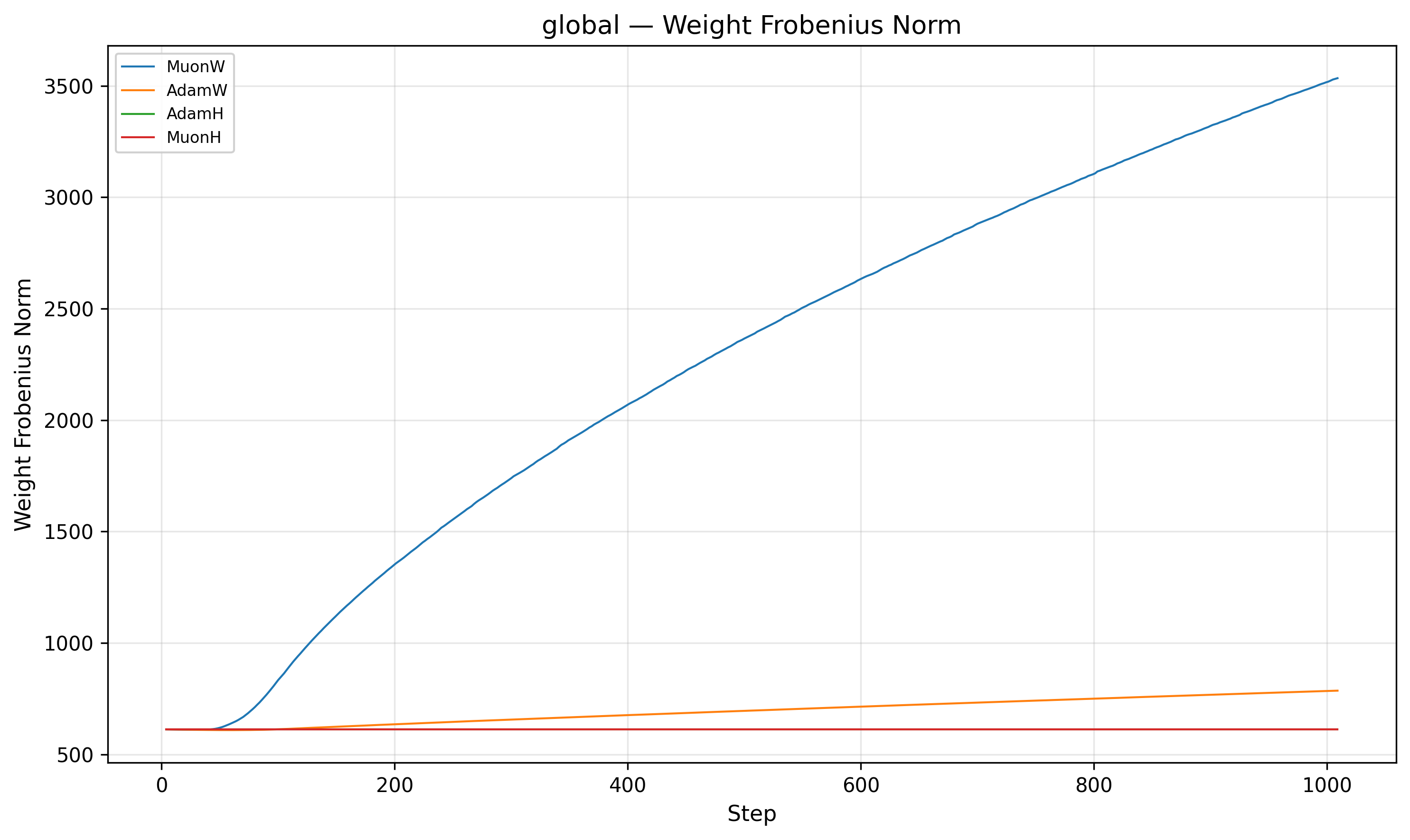
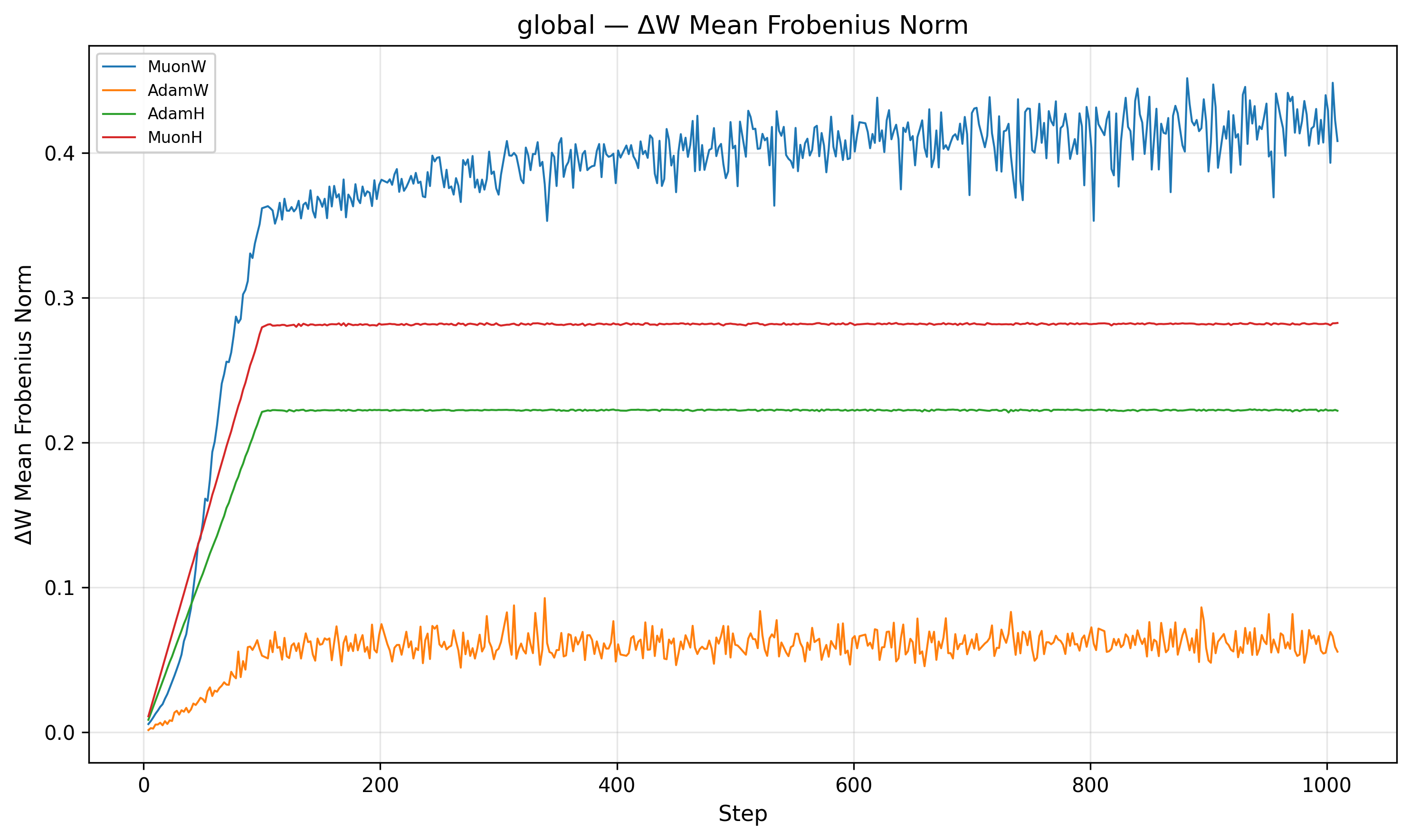
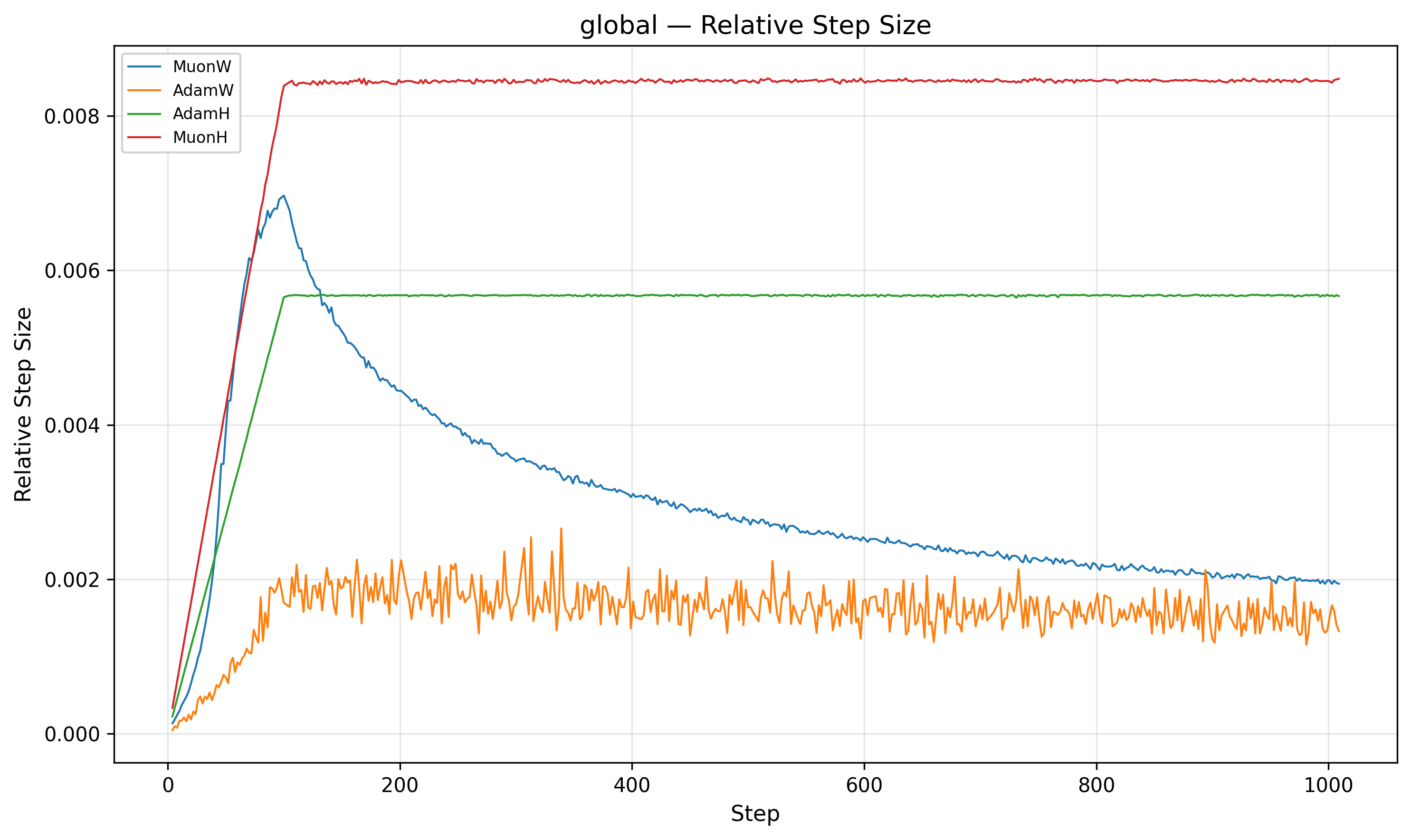
Indeed, MuonW's (Blue) weight norm grows monotonically throughout training. The update norm \(\|\Delta W\|\) is roughly constant post-warmup (it increases very slightly), but the weight denominator \(\|W\|\) balloons. Although independent weight decay should theoretically bound the norm at an equilibrium^{9, 10}, the norm continues to grow long after the nucleotide loss has begun to plateau. This causes the relative step size to decrease over training (driven mainly by weight norm growth), which may act like an implicit annealing schedule that helps the model refine its solution in later stages.

For MuonH (Red), the weight norm \(\|W\|\) is fixed. The relative step size flattens out and never decays. MuonH’s relative step size stays roughly constant; we suspect this limits fine-grained convergence by preventing late-stage refinement.

Activation Hacking: The Logit Inflation "Cheat"

There is an alternative, less flattering interpretation of MuonW's success: fit the cross-entropy loss by simply inflating the logits. In classification tasks, the cross-entropy loss can be decreased by sharpening the probability distribution (making the model more "confident"), even if the ranking of classes doesn't change.

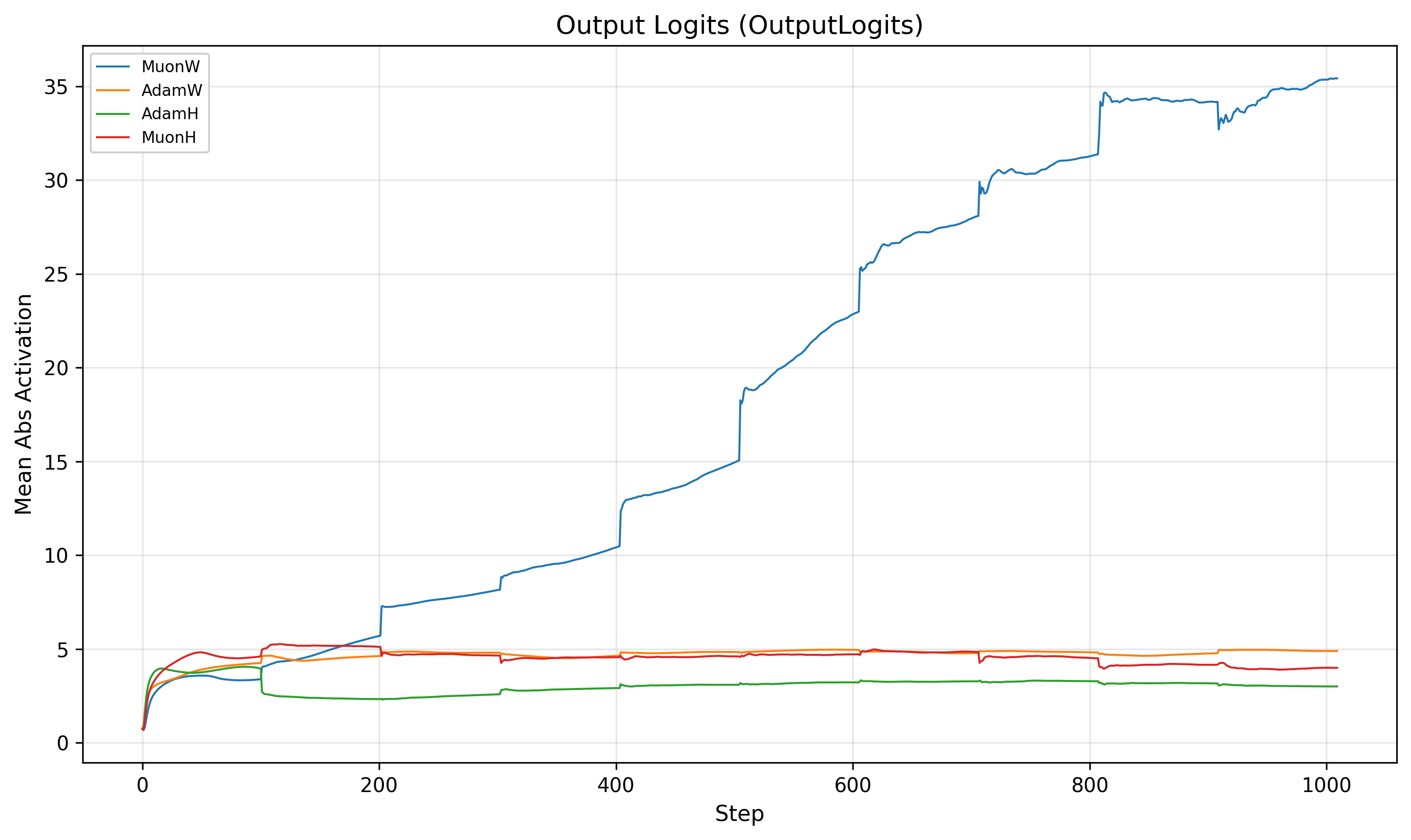
As noted above, MuonW's weight norm grows monotonically throughout training. While the RMSNorm-sandwiched hidden layers are scale invariant (Appendix F), the final output projection is not. There is no normalization between the last linear layer and the softmax. This means the runaway norm growth could potentially inflate the magnitude of the output logits, sharpening the softmax distribution and pushing the model toward higher confidence predictions.

This acts exactly like lowering the softmax temperature. Whether this "activation hacking" helps or hurts depends on the task. DNA has a vocabulary of just 4 bases, and in regulatory regions the correct nucleotide often dominates its context window. Sharper predictions on a tiny, low entropy vocabulary are frequently correct, so inflated logits often reduce cross-entropy loss in this setting. Natural language, by contrast, has a vocabulary of ~100k tokens with genuinely ambiguous contexts where probability mass must be spread across many plausible continuations¹⁵ Quantitatively, consider the softmax function \(\sigma(\mathbf{z})_i = \frac{e^{z_i}}{\sum_{j=1}^K e^{z_j}}\). If we multiply the logits by a large factor \(k\), the terms become \(e^{k z_i}\). Since the exponential function grows incredibly fast, even a small difference in raw logits becomes a massive difference after exponentiation. The largest logit \(z_i\) will dominate the sum in the denominator, pushing the probability \(\sigma(\mathbf{z})_i\) towards 1 (provided \(k\) is large enough).

For DNA (\(K=4\)), there are only 3 other terms in the denominator to compete with. Even a small lead for the correct nucleotide allows it to overwhelm the others; let \(k_{DNA}\) be the minimal such multiplier. For NLP (\(K \approx 100,000\)), the denominator sums over 100,000 other terms. Even if each is small, their total mass is significant, acting as a "drag" that prevents the correct token from dominating the distribution purely through scaling by \(k_{DNA}\). .

This means that part of MuonW's training loss advantage may be an artifact of the domain: the optimizer exploits the low cardinality and low entropy of the DNA vocabulary to "hack" the loss via logit scaling, rather than learning richer internal representations. In fact, MuonW's validation perplexity also clearly improved, which can also be explained by logit inflation! MuonH (Red), with its strict norm constraint, is mathematically forbidden from using this trick, which may partially explain its higher training loss despite learning a "cleaner" low-rank representation. Disentangling this effect from the genuine spectral capacity gains discussed above is an important open question, and one that a controlled comparison with a fixed norm output head could help resolve.

Thus, the results presented here reflect relative optimizer comparisons at a fixed compute budget, not the absolute frontier of model quality. Next, we plan to:

• Run the full sweep with SSO: repeat the Adam/Muon \(\times\) Hyperball sweeps using the Spectral Sphere Optimizer (SSO)¹⁸ to test whether controlling \(\sigma_1\) of the weight matrix directly improves stability and performance compared to Frobenius norm control.
• Explore hybrid optimizers: evaluate combinations of Muon and Adam updates (like PRISM¹⁹ and variants²⁰) and compare against these results.
• Evaluate on biological downstream tasks: measure whether perplexity gains translate to improvements on tasks that matter for biology, such as transcription factor motif recovery, and sequence generation.

References

- Loshchilov & Hutter. Fixing Weight Decay Regularization in Adam. arXiv 2017.
- Jordan et al. Muon: An optimizer for hidden layers in neural networks. 2024.
- Avsec et al. AlphaGenome: advancing regulatory variant effect prediction. bioRxiv 2025.
- Avsec et al. Effective gene expression prediction from sequence by integrating long range interactions. Nature Methods 2021.
- Brixi et al. Genome modeling and design across all domains of life with Evo 2. bioRxiv 2025.
- Chizat et al. On Lazy Training in Differentiable Programming. NeurIPS 2019.
- Jacot et al. Neural Tangent Kernel: Convergence and Generalization in Neural Networks. NeurIPS 2018.
- Jeremy Bernstein. The Modula Docs - Weight Erasure. 2025.
- Kosson et al. Rotational Equilibrium: How Weight Decay Balances Learning Across Neural Networks. ICML 2024.
- Wen et al. Fantastic Pretraining Optimizers and Where to Find Them II: From Weight Decay to Hyperball Optimization. 2025.
- Cesista. Muon and a Selective Survey on Steepest Descent in Riemannian and Non-Riemannian Manifolds. 2025.
- Bartlett et al. Spectrally-normalized margin bounds for neural networks. NeurIPS 2017.
- Zhang & Sennrich. Root Mean Square Layer Normalization. NeurIPS 2019.
- Gemma Team. Gemma 3 Technical Report. arXiv 2025.
- Jha & Reagen. NerVE: Nonlinear Eigenspectrum Dynamics in LLM Feed-Forward Networks. ICLR 2026.
- Gao et al. Representation Degeneration Problem in Training Natural Language Generation Models. ICLR 2019.
- Yang, Simon & Bernstein. A Spectral Condition for Feature Learning. arXiv 2023.
- Xie et al. Controlled LLM Training on Spectral Sphere. arXiv 2025.
- Yang. PRISM: Structured Optimization via Anisotropic Spectral Shaping. arXiv 2026.
- Cesista. Shampoo-PRISM: Kronecker-Factored Optimization via Anisotropic Spectral Shaping. 2026.
- Zach. The Concise Guide to Zipf’s Law. Statology.
- Piantadosi. Zipf’s word frequency law in natural language: A critical review and future directions. Psychonomic Bulletin & Review 2014.
- Wilson et al. The Marginal Value of Adaptive Gradient Methods in Machine Learning. NeurIPS 2017.
- Wolpert & Macready. No Free Lunch Theorems for Optimization. IEEE Trans. Evolutionary Computation 1997.